Date: Apr 21, 2026, Version: 0.1.2, Author: E. P. Metzner
Bessel functions
Calculating optical properties of small spherical particles heavily depends on the Bessel function after Friedrich Wilhelm Bessel. He analyzed the following differential equation with (complex) order \(\nu\) :
The functions, which solve this differential equation, are called the Bessel functions:
Bessel function of the first kind
\(J_{\nu}(z) \,=\, \sum_{m=0}^{\infty} (-1)^m \frac{m!}{\Gamma(m+\nu+1)} \left(\frac{x}{2}\right)^{2m+\nu}\)
Bessel function of the second kind
\(Y_{\nu}(z) \,=\, \frac{J_{\nu}(z)\cos(\nu\pi)-J_{-\nu}(z)}{\sin(\nu\pi)}\)
Bessel functions of the third kind, also called Hankel functions:
\(H_{\nu}^1(z) \,=\, J_{\nu}(z) + i Y_{\nu}(z)\)
\(H_{\nu}^2(z) \,=\, J_{\nu}(z) - i Y_{\nu}(z)\)
#import necessary modules
import numpy as np
if np.__version__>'1.25':
    np.set_printoptions(legacy="1.25", threshold=200)
import scipy.special as sp
import matplotlib.pyplot as plt
import matplotlib.gridspec as gridspec
plt.rcParams.update({"font.size":15, "figure.figsize":[16,9]})
import ARTmie as am
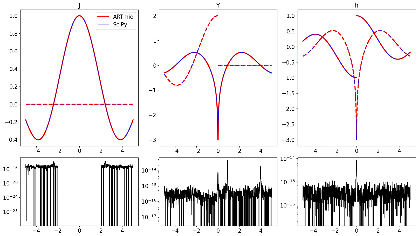
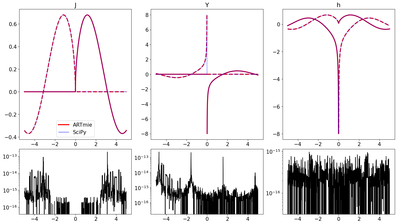
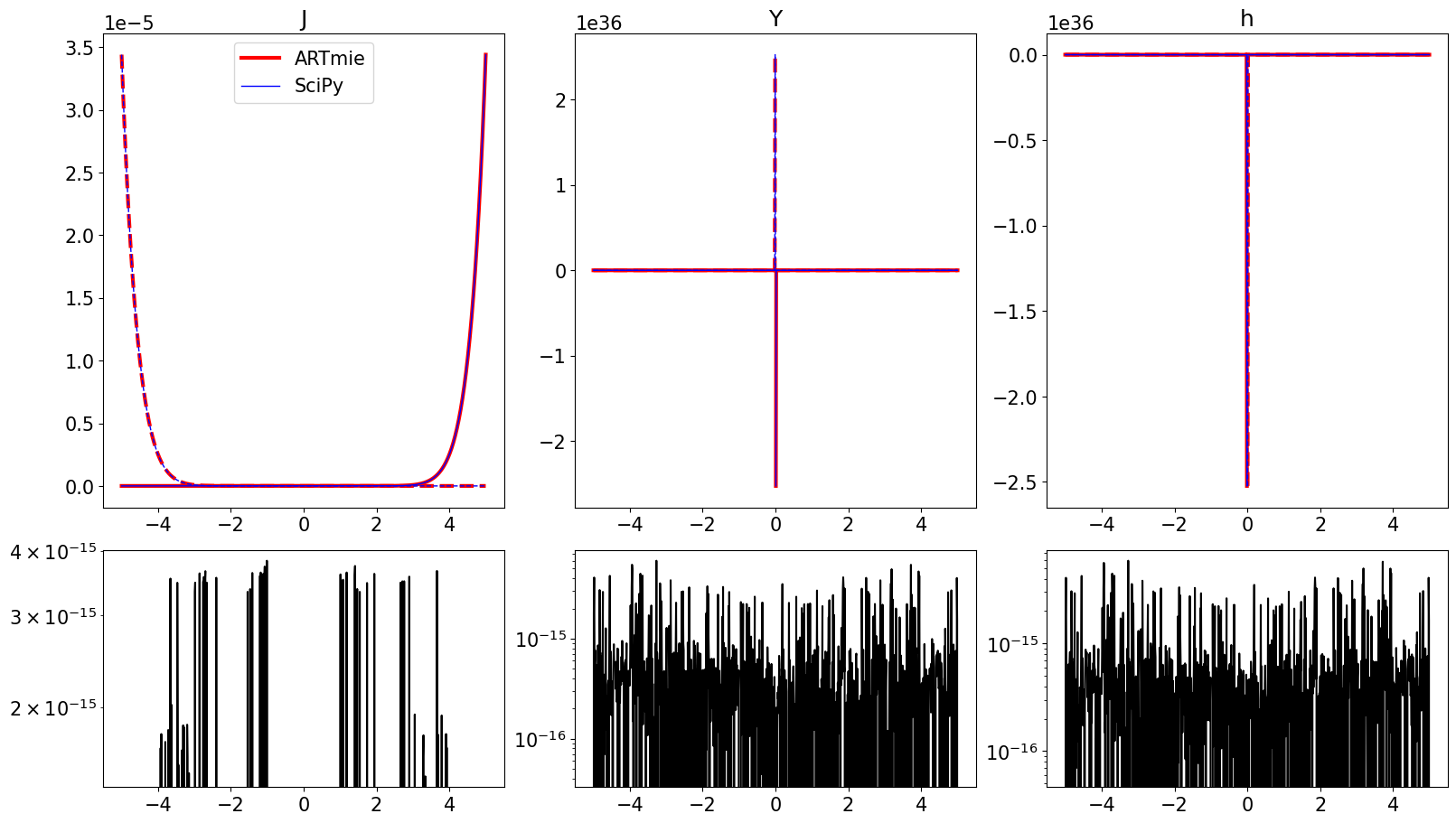
Let’s start with an evaluation of these Bessel function along the real axis
For basic visualisation, let us use 3 different orders of the Bessel function:
\(\nu = 0.0\)
\(\nu = 0.5\)
\(\nu = 12.5\)
The relative difference against the reference by SciPy is shown in black below.
x = np.linspace(-5.0, 5.0, 1001)
z = x + 0.0*1j

nu_list = [ 0.0, 0.5, 12.5 ]

for nu in nu_list:
    print(f'\n $\\nu$ = {nu}')
    am  = { 'J': ARTmie.besselj(nu, z),
            'Y': ARTmie.bessely(nu, z),
            'h': ARTmie.hankel(nu, z, 1) }
    ref = { 'J': sp.jv(nu, z),
            'Y': sp.yv(nu, z),
            'h': sp.hankel1(nu, z) }
    fig = plt.figure(constrained_layout=True)
    spec = gridspec.GridSpec(ncols=3, nrows=3, figure=fig)
    for i,k in enumerate(['J','Y','h']):
        axt = fig.add_subplot(spec[0:2, i:i+1])
        axl = fig.add_subplot(spec[2:3, i:i+1])
        axt.plot(x, np.real(am[k]),  color='#F00', ls='-',  lw=3, label='ARTmie')
        axt.plot(x, np.imag(am[k]),  color='#F00', ls='--', lw=3)
        axt.plot(x, np.real(ref[k]), color='#00F', ls='-',  lw=1, label='SciPy')
        axt.plot(x, np.imag(ref[k]), color='#00F', ls='--', lw=1)
        axt.set_title(k)
        if i==0:
            axt.legend()
        axl.plot(x, np.abs((am[k]-ref[k])/ref[k]), color='#000')
        axl.set_yscale('log')
    fig.show()
\(\nu = 0.0\)
\(\nu = 0.5\)
\(\nu = 12.5\)
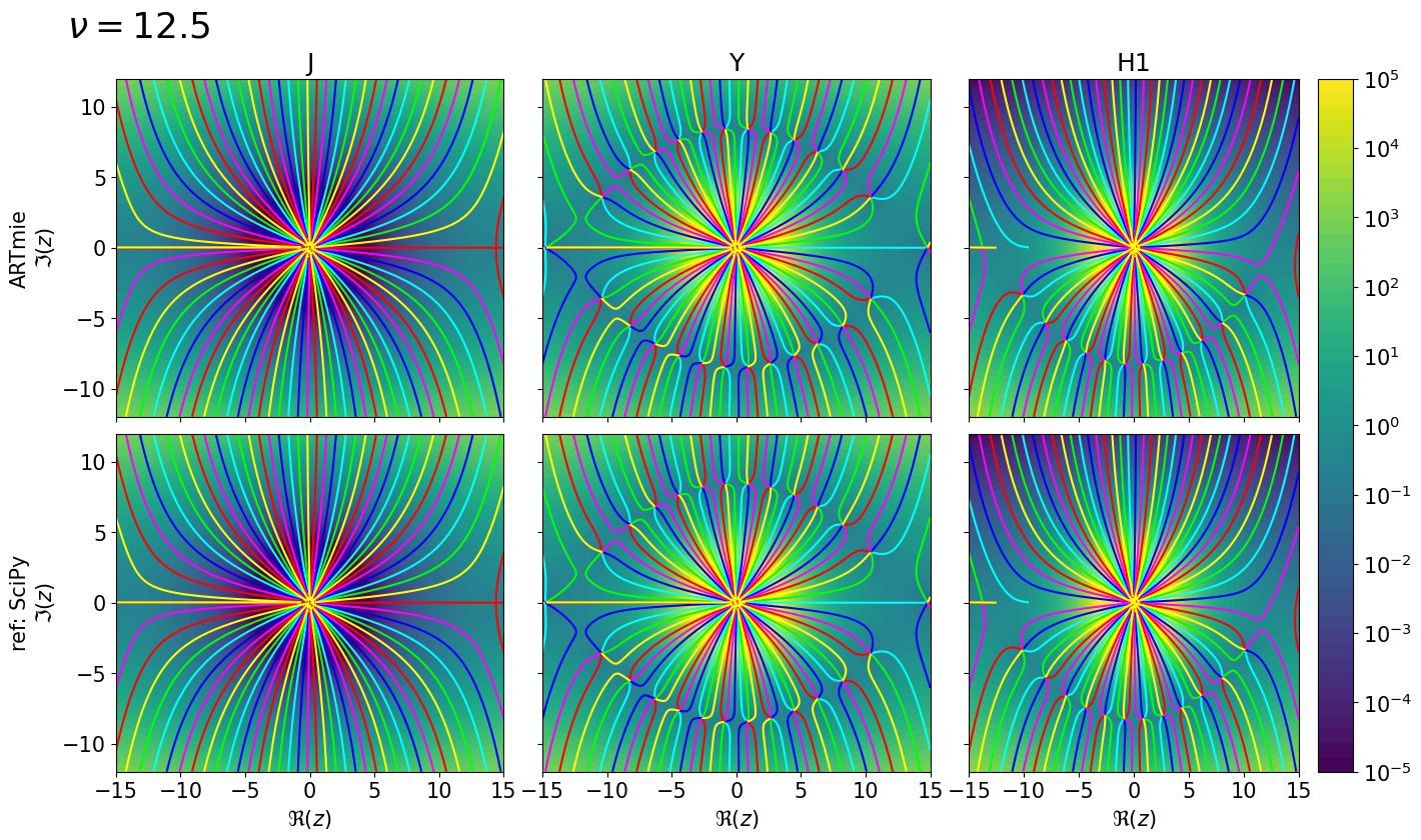
As the input to the Bessel functions is complex, let lock at a large range of complex numbers and compare again, how the Bessel functions behave against the reference by SciPy.
def plotCplx(ax, z, w, showPhase=True, view='value'):
    lev = np.linspace(-5.0,5.0,50)
    if view=='diff':
        lev = np.linspace(-16.0,-10.0,60)
    pmin,pmax = 10**lev[0],10**lev[-1]
    ab = np.abs(w)
    ab = np.log10(np.clip(ab, pmin+0.0*ab, pmax+0.0*ab))
    re,im = np.real(z),np.imag(z)
    cf = ax.contourf(re,im,ab,levels=lev);
    if showPhase:
        r2d = 180.0/np.pi
        ang = r2d*np.angle(w)
        ang2 = np.where(ang<0,ang+180,ang-180)
        ax.contour(re,im,np.where(np.abs(ang2)<=150,ang2,np.nan),levels=[-60,0,60],colors=[(0,1,0,1),(0,1,1,1),(0,0,1,1)])
        ax.contour(re,im,np.where(np.abs(ang)<=150,ang,np.nan),levels=[-60,0,60],colors=[(1,0,1,1),(1,0,0,1),(1,1,0,1)])
    return cf
for nu in nu_list:
    x = np.linspace(-10.0, 10.0, 500)*(1.0 if nu<10.0 else 1.5)
    y = np.linspace(-8.0, 8.0, 400)*(1.0 if nu<10.0 else 1.5)
    z = np.array([x+im*1j for im in y])
    am  = { 'J': np.array([ARTmie.besselj(nu, x+im*1j) for im in y]),
            'Y': np.array([ARTmie.bessely(nu, x+im*1j) for im in y]),
            'H1': np.array([ARTmie.hankel(nu, x+im*1j, 1) for im in y]) }
    ref = { 'J': sp.jv(nu, z),
            'Y': sp.yv(nu, z),
            'H1': sp.hankel1(nu, z) }
    fig,axs = plt.subplots(2,3,sharex=True,sharey=True)
    plt.subplots_adjust(wspace=0.10, hspace=0.05)
    for i,k in enumerate(['J','Y','H1']):
        #axt = fig.add_subplot(spec[0, i])
        #axl = fig.add_subplot(spec[1, i])
        axt,axl = axs[0,i],axs[1,i]
        p1 = plotCplx(axt, z, am[k])
        plotCplx(axl, z, ref[k])
        axt.set_title(k)
        if i==0:
            axt.annotate(f'$\\nu = {nu}$', (1.25*np.min(x),1.25*np.max(y)), annotation_clip=False, fontsize='xx-large')
            axt.set_ylabel('ARTmie\n$\Im(z)$')
            axl.set_ylabel('ref: SciPy\n$\Im(z)$')
        axl.set_xlabel('$\Re(z)$')
        if i==2:
            tt = [-5,-4,-3,-2,-1,0,1,2,3,4,5]
            ll = ["$10^{-5}$","$10^{-4}$","$10^{-3}$","$10^{-2}$","$10^{-1}$","$10^0$","$10^1$","$10^2$","$10^3$","$10^4$","$10^5$"]
            cb = fig.colorbar(p1, ax=[axt,axl], orientation='vertical', fraction=.1, ticks=tt)
            cb.ax.set_yticklabels(ll)
    fig.show()
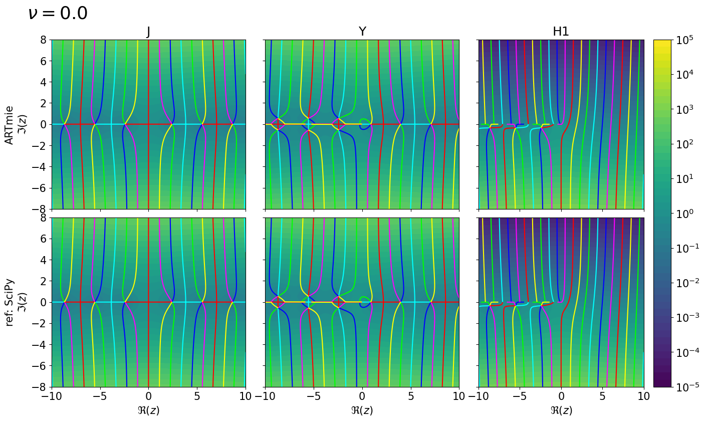

Mathematical accuracy
The Bessel functions are the mathematical basis for all Mie calculations.
Therefore, it is important that they are accurate.
Lets have a look, how good they are compaired to the implementation by SciPy here used as reference.
for nu in nu_list:
    x = np.linspace(-10.0, 10.0, 500)*(1.0 if nu<10.0 else 1.5)
    y = np.linspace(-8.0, 8.0, 400)*(1.0 if nu<10.0 else 1.5)
    z = np.array([x+im*1j for im in y])
    am  = { 'J': np.array([ARTmie.besselj(nu, x+im*1j) for im in y]),
            'Y': np.array([ARTmie.bessely(nu, x+im*1j) for im in y]),
            'H1': np.array([ARTmie.hankel(nu, x+im*1j, 1) for im in y]) }
    ref = { 'J': sp.jv(nu, z),
            'Y': sp.yv(nu, z),
            'H1': sp.hankel1(nu, z) }
    fig, axs = plt.subplots(1,3, figsize=(16,4), sharex=True, sharey=True)
    plt.subplots_adjust(wspace=0.10)
    for i,k in enumerate(['J','Y','H1']):
        p = plotCplx(axs[i], z, (am[k]-ref[k])/ref[k], showPhase=False, view='diff')
        axs[i].set_title(k)
        if i==0:
            axs[i].annotate(f'$\\nu = {nu}$', (1.25*np.min(x),1.25*np.max(y)), annotation_clip=False, fontsize='xx-large')
            axs[i].set_ylabel('$\\Im(z)$')
        axs[i].set_xlabel('$\\Re(z)$')
        if i==2:
            tt = [-16,-15,-14,-13,-12,-11,-10]
            ll = ["$10^{-16}$","$10^{-15}$","$10^{-14}$","$10^{-13}$","$10^{-12}$","$10^{-11}$","$10^{-10}$"]
            cb = fig.colorbar(p, ax=axs[i], orientation='vertical', fraction=.1, ticks=tt)
            cb.ax.set_yticklabels(ll)
    fig.suptitle('(ARTmie-SciPy)/SciPy', fontsize='x-large', y=1.03)
    fig.show()
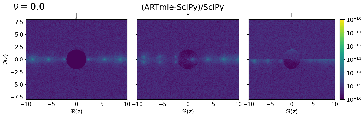
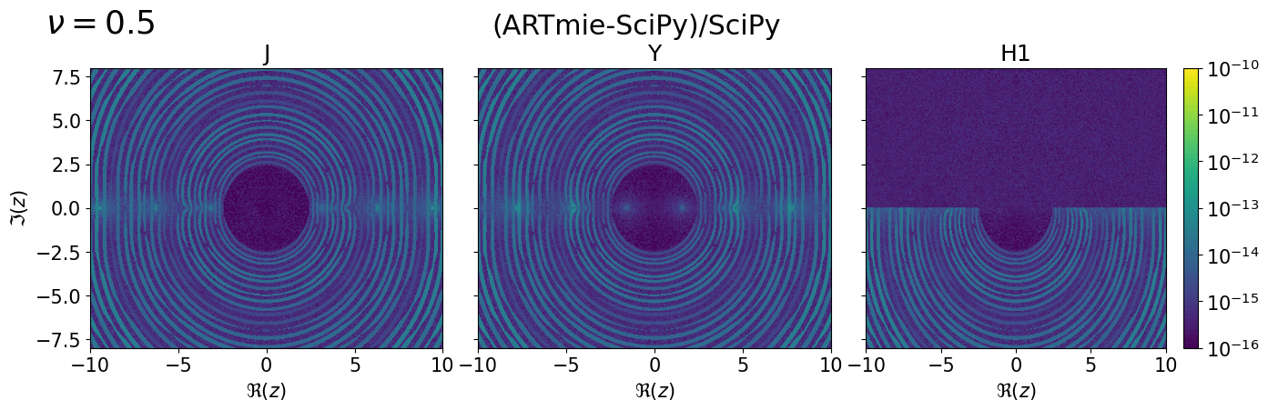
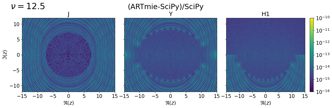
All differences are near the machine precision \((10^{-16} \sim 10^{-12})\).
Both implementations (ARTmie and SciPy) use the code by Amos [1] .
This explains the structures in the difference plots. Different regions of the complex number grid require different algorithms to converge quickly towards results with the best possible precision.