Date: Apr 21, 2026, Version: 0.1.2, Author: E. P. Metzner
Single particles
#imports
import numpy as np
if np.__version__>'1.25':
    np.set_printoptions(legacy="1.25", threshold=200)
import ARTmie
import matplotlib.pyplot as plt
plt.rcParams.update({"font.size":15, "figure.figsize":[16,9]})
- All starts with the core properties of single spherical object, which interacts with light:
diameter \(d\)
refractive index if the material \(m\)
- and the properties of the light, which interacts with the particle:
wavelength \(\lambda\)
ARTmie follows the convention to use nm for lengths and a positive sign for the extinction part of the complex refractive index \(m=n+i\cdot{}k\)
Assume a water sphere of 50µm diameter. Red light of 650nm shines on these water droplet, setting its refractive index to \(m=1.331+i\cdot{}1.64×10^{−8}\) (see wikipedia) From this, the “size parameter” \(x=\pi\frac{d}{\lambda}\)
#refractive index of water
def ri_h2o(wl,t_celsius,rho_kgm3):
    t,r,luv2,lir2 = (273.15+t_celsius)/273.15,rho_kgm3/1000.0,0.2292020**2,5.432937**2
    l2 = (wl/589.0)**2
    re = (0.244257733 + 0.00974634476*r - 0.00373234996*t + 0.000268678472*l2*t + 0.0015820570/l2 + 0.00245934259/(l2 - luv2) + 0.900704920/(l2 - lir2) - 0.0166626219*r*r)*r
    im = -4.0 - 4.71/(1.0 + 3.7e-6*(wl-255)**2 - 1.0e-3*(wl-255)) #log10(k), eye-balled approx. of fig 1 in https://www.researchgate.net/publication/286477328_Dual-wavelength_light-scattering_technique_for_selective_detection_of_volcanic_ash_particles_in_the_presence_of_water_droplets/figures?lo=1
    return np.sqrt((1+re+re)/(1-re)) + (10**im)*1j

#basic properties
diam  = 50000.0
wl    = 650.0
m_h2o = ri_h2o(wl, 25.0, 997.0)
ARTmie gives you the external field coefficients \(a_n\) and \(b_n\). They are calculated according to the formulae after Gustav Mie and related work of e.g. Ludvig Lorenz and Peter Debey. (here shown for non-magnetic materials \(\mu_r=1\) and assuming \(n=1+0i\) for the environment):
They take heavily use of the spherical bessel functions \(j_n()\) and \(h_n^1()\) after mathematician Friedrich Wilhelm Bessel.
x = np.pi*diam/wl
an,bn = ARTmie.Mie_ab(m_h2o,x)
print('a_n =',an)
print('b_n =',bn)
a_n = [9.68060554e-01-1.75830088e-01j 9.99877543e-01-1.09760102e-02j
 9.67565189e-01-1.77143092e-01j ... 2.39383064e-13+7.35395440e-08j
 6.23218056e-12+3.34007256e-07j 5.70101814e-14-1.96026838e-08j]
b_n = [9.99940686e-01-7.57218172e-03j 9.67851760e-01-1.76384874e-01j
 9.99739720e-01-1.60701063e-02j ... 1.29269903e-13+6.93833022e-08j
 2.77636435e-13+7.42606651e-08j 2.39137530e-13-3.54725158e-08j]
- From these external field coefficients, ARTmie can calculate the Mie efficiencies
Qext: extinction
Qsca: scattering
Qabs: absorption
Qback: backscattering
Qratio: backscatter-ratio Qback/Qsca
Qpr: radiation pressure
g: scattering asymmetry (positive for increased forward scattering, negative for more backward scattering)
Those can be calculated as follows from the external field coefficients \(a_n\) and \(b_n\):
where * denotes complex conjugates.
q = ARTmie.ab2mie(an,bn,wl,diam, asDict=True)
print(q)
{'Qext': 2.050656595072554, 'Qsca': 2.05064626624816, 'Qabs': 1.0328824394001401e-05, 'Qback': 3.001738464591244, 'Qratio': 1.4638011996497045, 'Qpr': 0.26224549828037075, 'g': 0.8721207193204709}
Those can be calculated directly with the call ARTmie.MieQ().
The option asCrossSection gives you the resalt as scattering cross section in \(\text{nm}^2\).
Backscatter-ratio and asymmetry parameter stay dimensionless.
c = ARTmie.MieQ(m_h2o, diam, wl, asCrossSection=True, asDict=True)
print(c)
{'Cext': 4026454808.8221216, 'Csca': 4026434528.222849, 'Cabs': 20280.599272758656, 'Cback': 5893899692.7235985, 'Cratio': 1.4638011996497045, 'Cpr': 514917831.77162963, 'g': 0.8721207193204709}
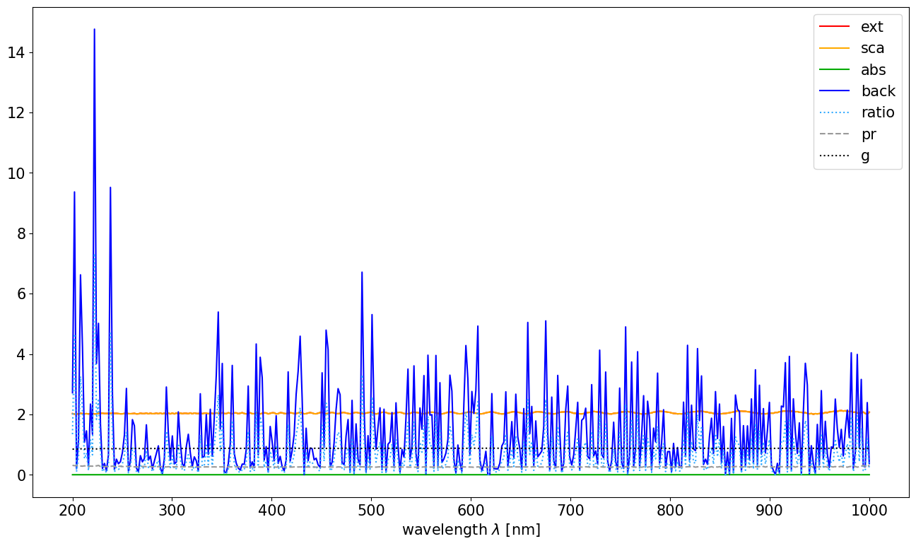
It is also possible to calculate this optical properties for a whole range of wavelengths simultaneously. So let us consider the (very wide) optical range from 200nm to 1000nm:
#calculate optical properties
wl = np.linspace(200.0, 1000.0, 400)
m_h2o = ri_h2o(wl, 25.0, 997.0)

q = ARTmie.MieQ(m_h2o, diam, wl, asDict=True)

#plot results
plt.figure()
plt.plot(wl, q['Qext'],   color='#F00', ls='-',  label='ext')
plt.plot(wl, q['Qsca'],   color='#FA0', ls='-',  label='sca')
plt.plot(wl, q['Qabs'],   color='#0A0', ls='-',  label='abs')
plt.plot(wl, q['Qback'],  color='#00F', ls='-',  label='back')
plt.plot(wl, q['Qratio'], color='#3AF', ls=':',  label='ratio')
plt.plot(wl, q['Qpr'],    color='#999', ls='--', label='pr')
plt.plot(wl, q['g'],      color='#000', ls=':',  label='g')
plt.legend()
plt.xlabel('wavelength $\\lambda$ [nm]')
plt.show()
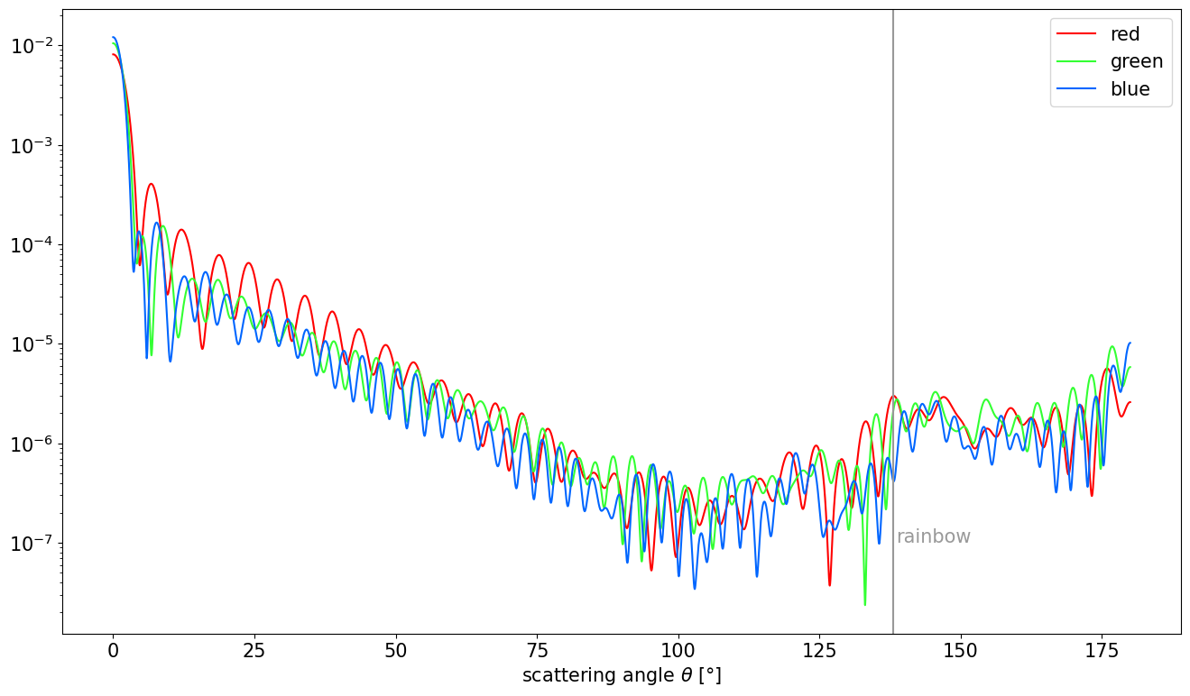
Furthermore scattering can also be calculated dependend on the scattering angle.
For this, ARTmie provides the function ARTmie.ScatteringFunction().
#choosing three representative wavelengths and corresponding refractive indices to visualize the rainbow near 138° (180°-42°)
#wavelengths are picked for good measure from https://en.wikipedia.org/wiki/Visible_spectrum
diam = 9108.0 #9.108µm
w_red, m_red = 700.0, ri_h2o(700.0, 25.0, 997.0)
w_grn, m_grn = 550.0, ri_h2o(550.0, 25.0, 997.0)
w_blu, m_blu = 470.0, ri_h2o(470.0, 25.0, 997.0)

theta = np.linspace(0.0, 180.0, 9000)
d2r = np.pi/180.0

sl_red,sr_red,su_red = ARTmie.ScatteringFunction(m_red,diam,w_red,theta*d2r)
sl_grn,sr_grn,su_grn = ARTmie.ScatteringFunction(m_grn,diam,w_grn,theta*d2r)
sl_blu,sr_blu,su_blu = ARTmie.ScatteringFunction(m_blu,diam,w_blu,theta*d2r)

#normalizing
su_red /= np.sum(su_red)
su_grn /= np.sum(su_grn)
su_blu /= np.sum(su_blu)

plt.figure()
plt.plot(theta, su_red, color='#F00', label='red')
plt.plot(theta, su_grn, color='#3F3', label='green')
plt.plot(theta, su_blu, color='#06F', label='blue')
plt.gca().set_yscale('log')
plt.axvline(138.0, color='#999')
plt.annotate('rainbow', xy=(138.5,10**-7), color='#999')
plt.legend()
plt.xlabel('scattering angle $\\theta$ [°]')
plt.show()